2.1. Continuous Optimization

surrogate.benchmarks.cigar(variable)

Cigar test objective function.

Type	minimization
Range	none
Global optima	\(x_i = 0, \forall i \in \lbrace 1 \ldots N\rbrace\), \(f(\mathbf{x}) = 0\)
Function	\(f(\mathbf{x}) = x_0^2 + 10^6\sum_{i=1}^N\,x_i^2\)

surrogate.benchmarks.plane(variable)

Plane test objective function.

Type	minimization
Range	none
Global optima	\(x_i = 0, \forall i \in \lbrace 1 \ldots N\rbrace\), \(f(\mathbf{x}) = 0\)
Function	\(f(\mathbf{x}) = x_0\)

surrogate.benchmarks.sphere(variable)

Sphere test objective function.

Type	minimization
Range	none
Global optima	\(x_i = 0, \forall i \in \lbrace 1 \ldots N\rbrace\), \(f(\mathbf{x}) = 0\)
Function	\(f(\mathbf{x}) = \sum_{i=1}^Nx_i^2\)

surrogate.benchmarks.rand(variable)

Random test objective function.

Type	minimization or maximization
Range	none
Global optima	none
Function	\(f(\mathbf{x}) = \text{\texttt{random}}(0,1)\)

surrogate.benchmarks.ackley(variable)

Ackley test objective function.

Type	minimization
Range	\(x_i \in [-15, 30]\)
Global optima	\(x_i = 0, \forall i \in \lbrace 1 \ldots N\rbrace\), \(f(\mathbf{x}) = 0\)
Function	\(f(\mathbf{x}) = 20 - 20\exp\left(-0.2\sqrt{\frac{1}{N} \sum_{i=1}^N x_i^2} \right) + e - \exp\left(\frac{1}{N}\sum_{i=1}^N \cos(2\pi x_i) \right)\)

(Source code, png, hires.png, pdf)

surrogate.benchmarks.bohachevsky(variable)

Bohachevsky test objective function.

Type	minimization
Range	\(x_i \in [-100, 100]\)
Global optima	\(x_i = 0, \forall i \in \lbrace 1 \ldots N\rbrace\), \(f(\mathbf{x}) = 0\)
Function	\(f(\mathbf{x}) = \sum_{i=1}^{N-1}(x_i^2 + 2x_{i+1}^2 - 0.3\cos(3\pi x_i) - 0.4\cos(4\pi x_{i+1}) + 0.7)\)

(Source code, png, hires.png, pdf)

surrogate.benchmarks.griewank(variable)

Griewank test objective function.

Type	minimization
Range	\(x_i \in [-600, 600]\)
Global optima	\(x_i = 0, \forall i \in \lbrace 1 \ldots N\rbrace\), \(f(\mathbf{x}) = 0\)
Function	\(f(\mathbf{x}) = \frac{1}{4000}\sum_{i=1}^N\,x_i^2 - \prod_{i=1}^N\cos\left(\frac{x_i}{\sqrt{i}}\right) + 1\)

(Source code, png, hires.png, pdf)

surrogate.benchmarks.h1(variable)

Simple two-dimensional function containing several local maxima. From: The Merits of a Parallel Genetic Algorithm in Solving Hard Optimization Problems, A. J. Knoek van Soest and L. J. R. Richard Casius, J. Biomech. Eng. 125, 141 (2003)

Type	maximization
Range	\(x_i \in [-100, 100]\)
Global optima	\(\mathbf{x} = (8.6998, 6.7665)\), \(f(\mathbf{x}) = 2\)
Function	\(f(\mathbf{x}) = \frac{\sin(x_1 - \frac{x_2}{8})^2 + \sin(x_2 + \frac{x_1}{8})^2}{\sqrt{(x_1 - 8.6998)^2 + (x_2 - 6.7665)^2} + 1}\)

(Source code, png, hires.png, pdf)

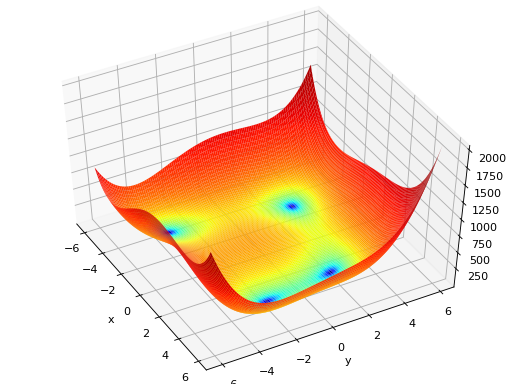
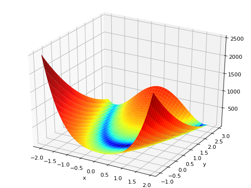
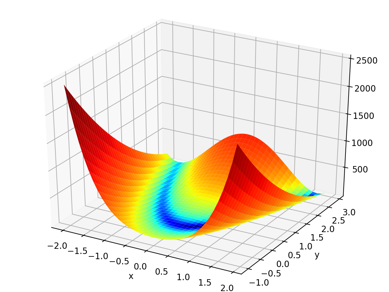
surrogate.benchmarks.himmelblau(variable)

The Himmelblau’s function is multimodal with 4 defined minimums in \([-6, 6]^2\).

Type	minimization
Range	\(x_i \in [-6, 6]\)
Global optima	\(\mathbf{x}_1 = (3.0, 2.0)\), \(f(\mathbf{x}_1) = 0\) \(\mathbf{x}_2 = (-2.805118, 3.131312)\), \(f(\mathbf{x}_2) = 0\) \(\mathbf{x}_3 = (-3.779310, -3.283186)\), \(f(\mathbf{x}_3) = 0\) \(\mathbf{x}_4 = (3.584428, -1.848126)\), \(f(\mathbf{x}_4) = 0\)
Function	\(f(x_1, x_2) = (x_1^2 + x_2 - 11)^2 + (x_1 + x_2^2 -7)^2\)

(Source code, png, hires.png, pdf)

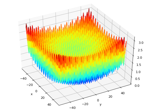
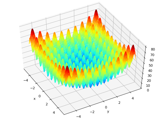
surrogate.benchmarks.rastrigin(variable)

Rastrigin test objective function.

Type	minimization
Range	\(x_i \in [-5.12, 5.12]\)
Global optima	\(x_i = 0, \forall i \in \lbrace 1 \ldots N\rbrace\), \(f(\mathbf{x}) = 0\)
Function	\(f(\mathbf{x}) = 10N \sum_{i=1}^N x_i^2 - 10 \cos(2\pi x_i)\)

(Source code, png, hires.png, pdf)

surrogate.benchmarks.rastrigin_scaled(variable)

Scaled Rastrigin test objective function.

\(f_{\text{RastScaled}}(\mathbf{x}) = 10N + \sum_{i=1}^N \left(10^{\left(\frac{i-1}{N-1}\right)} x_i \right)^2 x_i)^2 - 10\cos\left(2\pi 10^{\left(\frac{i-1}{N-1}\right)} x_i \right)\)

surrogate.benchmarks.rastrigin_skew(variable)

Skewed Rastrigin test objective function.

\(f_{\text{RastSkew}}(\mathbf{x}) = 10N \sum_{i=1}^N \left(y_i^2 - 10 \cos(2\pi x_i)\right)\)

\(\text{with } y_i = \begin{cases} 10\cdot x_i & \text{ if } x_i > 0,\\ x_i & \text{ otherwise } \end{cases}\)

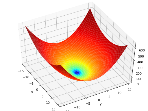
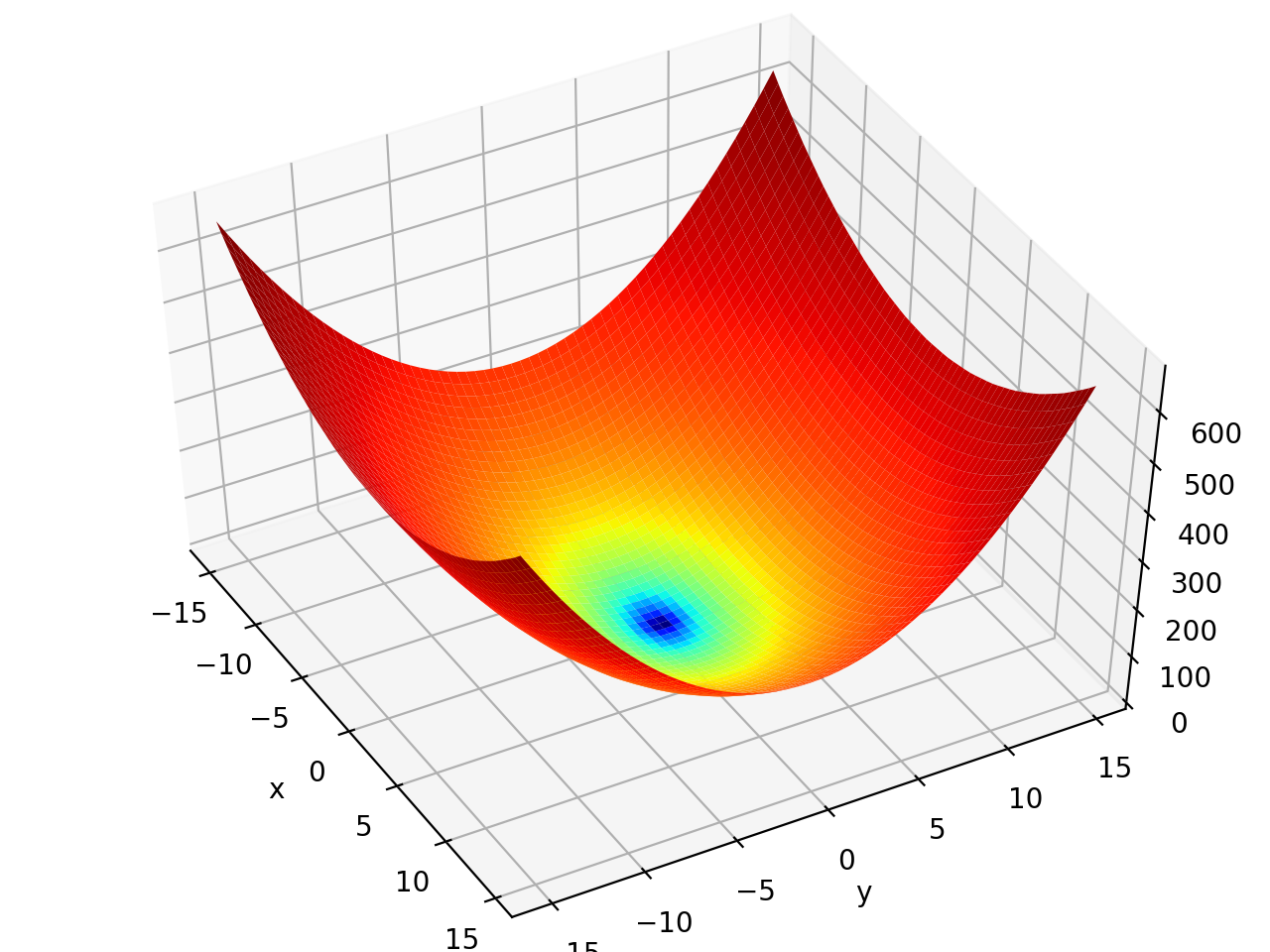
surrogate.benchmarks.rosenbrock(variable)

Rosenbrock test objective function.

Type	minimization
Range	none
Global optima	\(x_i = 1, \forall i \in \lbrace 1 \ldots N\rbrace\), \(f(\mathbf{x}) = 0\)
Function	\(f(\mathbf{x}) = \sum_{i=1}^{N-1} (1-x_i)^2 + 100 (x_{i+1} - x_i^2 )^2\)

(Source code, png, hires.png, pdf)

surrogate.benchmarks.schaffer(variable)

Schaffer test objective function.

Type	minimization
Range	\(x_i \in [-100, 100]\)
Global optima	\(x_i = 0, \forall i \in \lbrace 1 \ldots N\rbrace\), \(f(\mathbf{x}) = 0\)
Function	\(f(\mathbf{x}) = \sum_{i=1}^{N-1} (x_i^2+x_{i+1}^2)^{0.25} \cdot \left[ \sin^2(50\cdot(x_i^2+x_{i+1}^2)^{0.10}) + 1.0 \right]\)

(Source code, png, hires.png, pdf)

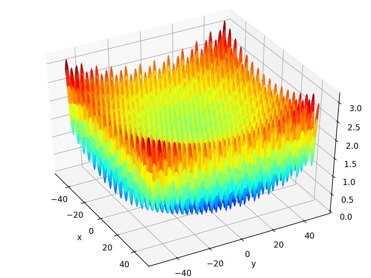
surrogate.benchmarks.schwefel(variable)

Schwefel test objective function.

Type	minimization
Range	\(x_i \in [-500, 500]\)
Global optima	\(x_i = 420.96874636, \forall i \in \lbrace 1 \ldots N\rbrace\), \(f(\mathbf{x}) = 0\)
Function	\(f(\mathbf{x}) = 418.9828872724339\cdot N - \sum_{i=1}^N\,x_i\sin\left(\sqrt{|x_i|}\right)\)

(Source code, png, hires.png, pdf)

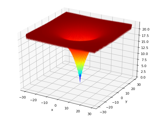
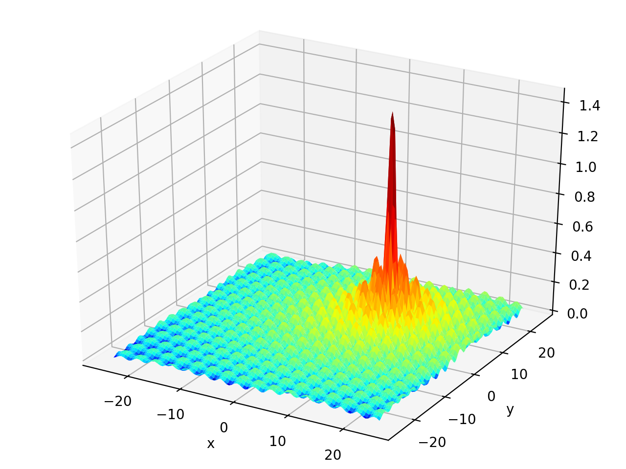
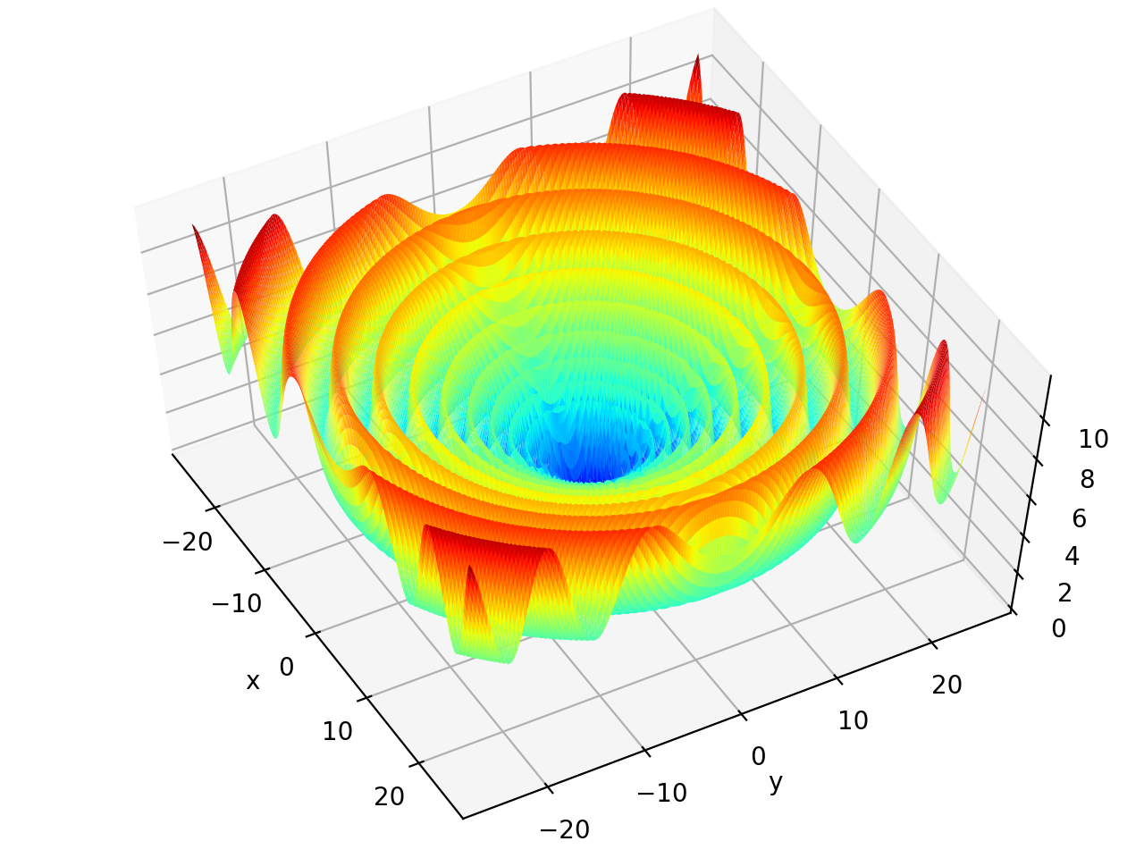
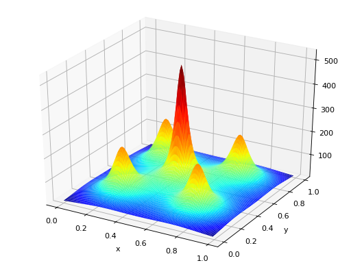
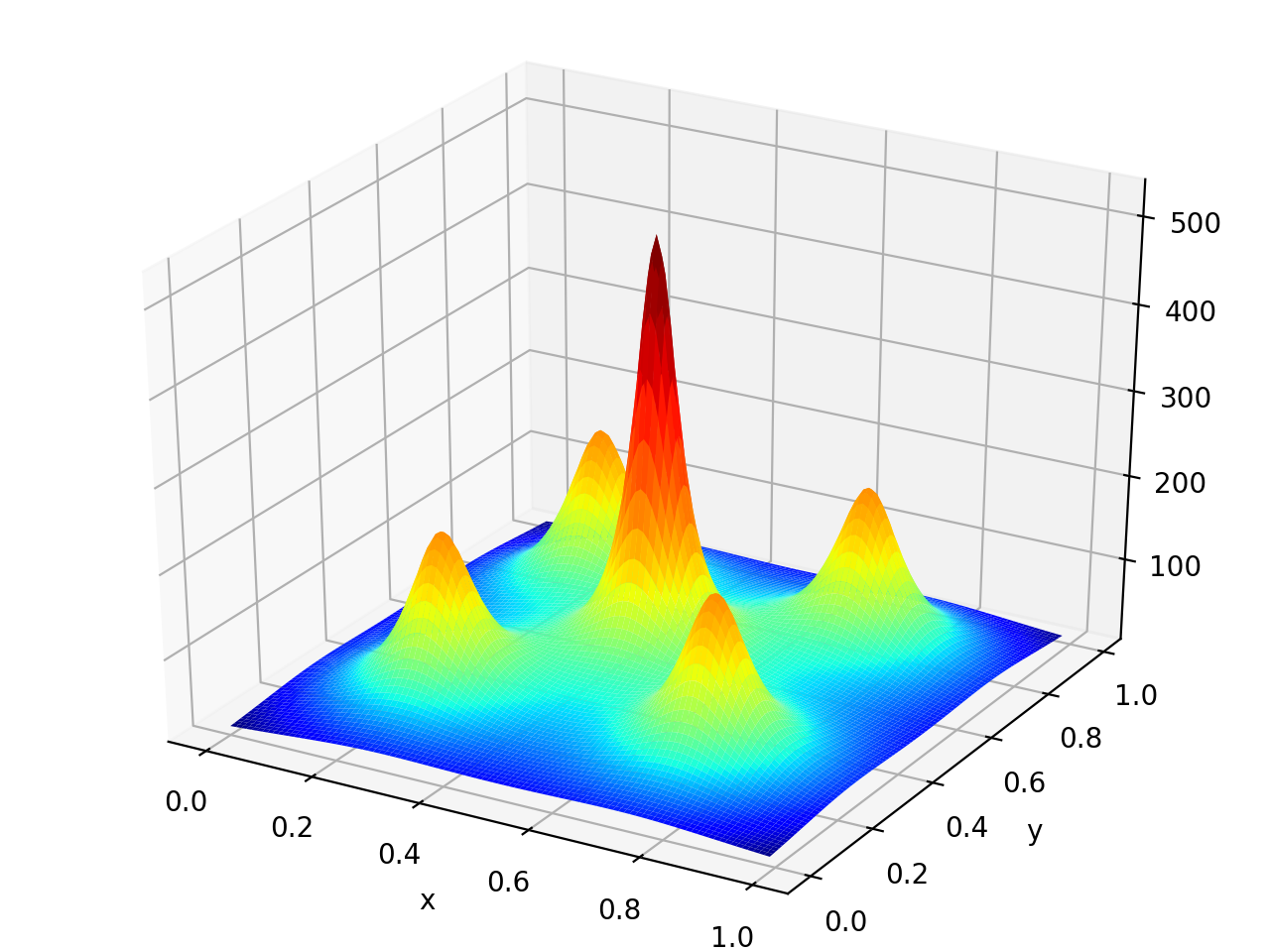
surrogate.benchmarks.shekel(variable, a, c)

The Shekel multimodal function can have any number of maxima. The number of maxima is given by the length of any of the arguments a or c, a is a matrix of size \(M\times N\), where M is the number of maxima and N the number of dimensions and c is a \(M\times 1\) vector. The matrix \(\mathcal{A}\) can be seen as the position of the maxima and the vector \(\mathbf{c}\), the width of the maxima.

\(f_\text{Shekel}(\mathbf{x}) = \sum_{i = 1}^{M} \frac{1}{c_{i} + \sum_{j = 1}^{N} (x_{j} - a_{ij})^2 }\)

The following figure uses

\(\mathcal{A} = \begin{bmatrix} 0.5 & 0.5 \\ 0.25 & 0.25 \\ 0.25 & 0.75 \\ 0.75 & 0.25 \\ 0.75 & 0.75 \end{bmatrix}\) and \(\mathbf{c} = \begin{bmatrix} 0.002 \\ 0.005 \\ 0.005 \\ 0.005 \\ 0.005 \end{bmatrix}\), thus defining 5 maximums in \(\mathbb{R}^2\).

(Source code, png, hires.png, pdf)

2.2. Multi-objective

surrogate.benchmarks.fonseca(variable)

Fonseca and Fleming’s multiobjective function. From: C. M. Fonseca and P. J. Fleming, “Multiobjective optimization and multiple constraint handling with evolutionary algorithms – Part II: Application example”, IEEE Transactions on Systems, Man and Cybernetics, 1998.

\(f_{\text{Fonseca}1}(\mathbf{x}) = 1 - e^{-\sum_{i=1}^{3}(x_i - \frac{1}{\sqrt{3}})^2}\)

\(f_{\text{Fonseca}2}(\mathbf{x}) = 1 - e^{-\sum_{i=1}^{3}(x_i + \frac{1}{\sqrt{3}})^2}\)

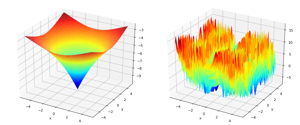
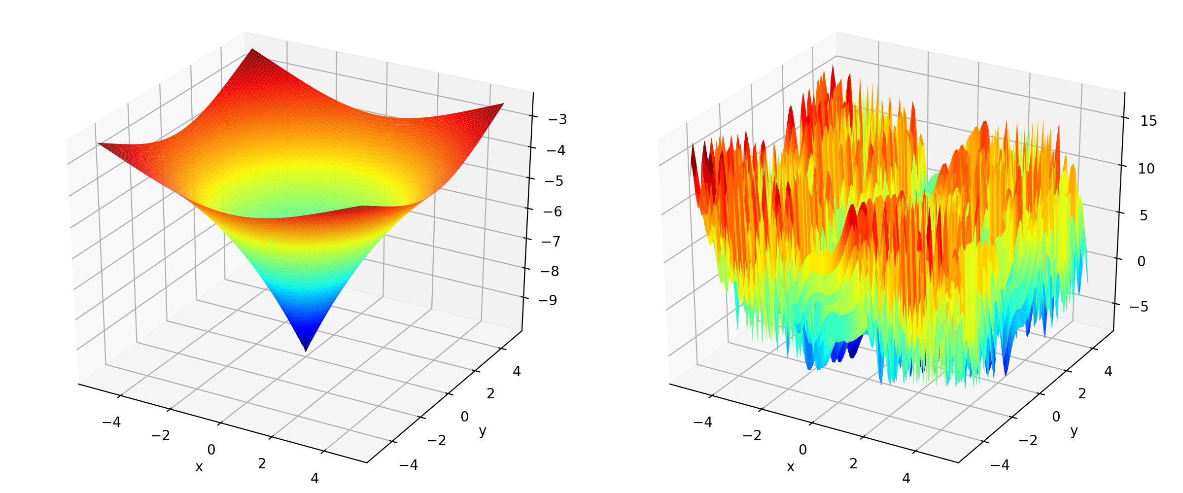
surrogate.benchmarks.kursawe(variable)

Kursawe multiobjective function.

\(f_{\text{Kursawe}1}(\mathbf{x}) = \sum_{i=1}^{N-1} -10 e^{-0.2 \sqrt{x_i^2 + x_{i+1}^2} }\)

\(f_{\text{Kursawe}2}(\mathbf{x}) = \sum_{i=1}^{N} |x_i|^{0.8} + 5 \sin(x_i^3)\)

(Source code, png, hires.png, pdf)

surrogate.benchmarks.schaffer_mo(variable)

Schaffer’s multiobjective function on a one attribute variable. From: J. D. Schaffer, “Multiple objective optimization with vector evaluated genetic algorithms”, in Proceedings of the First International Conference on Genetic Algorithms, 1987.

\(f_{\text{Schaffer}1}(\mathbf{x}) = x_1^2\)

\(f_{\text{Schaffer}2}(\mathbf{x}) = (x_1-2)^2\)

surrogate.benchmarks.dtlz1(variable, obj)

DTLZ1 mutliobjective function. It returns a tuple of obj values. The variable must have at least obj elements. From: K. Deb, L. Thiele, M. Laumanns and E. Zitzler. Scalable Multi-Objective Optimization Test Problems. CEC 2002, p. 825 - 830, IEEE Press, 2002.

\(g(\mathbf{x}_m) = 100\left(|\mathbf{x}_m| + \sum_{x_i \in \mathbf{x}_m}\left((x_i - 0.5)^2 - \cos(20\pi(x_i - 0.5))\right)\right)\)

\(f_{\text{DTLZ1}1}(\mathbf{x}) = \frac{1}{2} (1 + g(\mathbf{x}_m)) \prod_{i=1}^{m-1}x_i\)

\(f_{\text{DTLZ1}2}(\mathbf{x}) = \frac{1}{2} (1 + g(\mathbf{x}_m)) (1-x_{m-1}) \prod_{i=1}^{m-2}x_i\)

\(\ldots\)

\(f_{\text{DTLZ1}m-1}(\mathbf{x}) = \frac{1}{2} (1 + g(\mathbf{x}_m)) (1 - x_2) x_1\)

\(f_{\text{DTLZ1}m}(\mathbf{x}) = \frac{1}{2} (1 - x_1)(1 + g(\mathbf{x}_m))\)

Where \(m\) is the number of objectives and \(\mathbf{x}_m\) is a vector of the remaining attributes \([x_m~\ldots~x_n]\) of the variable in \(n > m\) dimensions.

surrogate.benchmarks.dtlz2(variable, obj)

DTLZ2 mutliobjective function. It returns a tuple of obj values. The variable must have at least obj elements. From: K. Deb, L. Thiele, M. Laumanns and E. Zitzler. Scalable Multi-Objective Optimization Test Problems. CEC 2002, p. 825 - 830, IEEE Press, 2002.

\(g(\mathbf{x}_m) = \sum_{x_i \in \mathbf{x}_m} (x_i - 0.5)^2\)

\(f_{\text{DTLZ2}1}(\mathbf{x}) = (1 + g(\mathbf{x}_m)) \prod_{i=1}^{m-1} \cos(0.5x_i\pi)\)

\(f_{\text{DTLZ2}2}(\mathbf{x}) = (1 + g(\mathbf{x}_m)) \sin(0.5x_{m-1}\pi ) \prod_{i=1}^{m-2} \cos(0.5x_i\pi)\)

\(\ldots\)

\(f_{\text{DTLZ2}m}(\mathbf{x}) = (1 + g(\mathbf{x}_m)) \sin(0.5x_{1}\pi )\)

Where \(m\) is the number of objectives and \(\mathbf{x}_m\) is a vector of the remaining attributes \([x_m~\ldots~x_n]\) of the variable in \(n > m\) dimensions.

surrogate.benchmarks.dtlz3(variable, obj)

DTLZ3 mutliobjective function. It returns a tuple of obj values. The variable must have at least obj elements. From: K. Deb, L. Thiele, M. Laumanns and E. Zitzler. Scalable Multi-Objective Optimization Test Problems. CEC 2002, p. 825 - 830, IEEE Press, 2002.

\(g(\mathbf{x}_m) = 100\left(|\mathbf{x}_m| + \sum_{x_i \in \mathbf{x}_m}\left((x_i - 0.5)^2 - \cos(20\pi(x_i - 0.5))\right)\right)\)

\(f_{\text{DTLZ3}1}(\mathbf{x}) = (1 + g(\mathbf{x}_m)) \prod_{i=1}^{m-1} \cos(0.5x_i\pi)\)

\(f_{\text{DTLZ3}2}(\mathbf{x}) = (1 + g(\mathbf{x}_m)) \sin(0.5x_{m-1}\pi ) \prod_{i=1}^{m-2} \cos(0.5x_i\pi)\)

\(\ldots\)

\(f_{\text{DTLZ3}m}(\mathbf{x}) = (1 + g(\mathbf{x}_m)) \sin(0.5x_{1}\pi )\)

Where \(m\) is the number of objectives and \(\mathbf{x}_m\) is a vector of the remaining attributes \([x_m~\ldots~x_n]\) of the variable in \(n > m\) dimensions.

surrogate.benchmarks.dtlz4(variable, obj, alpha)

DTLZ4 mutliobjective function. It returns a tuple of obj values. The variable must have at least obj elements. The alpha parameter allows for a meta-variable mapping in dtlz2() \(x_i \rightarrow x_i^\alpha\), the authors suggest \(\alpha = 100\). From: K. Deb, L. Thiele, M. Laumanns and E. Zitzler. Scalable Multi-Objective Optimization Test Problems. CEC 2002, p. 825 - 830, IEEE Press, 2002.

\(g(\mathbf{x}_m) = \sum_{x_i \in \mathbf{x}_m} (x_i - 0.5)^2\)

\(f_{\text{DTLZ4}1}(\mathbf{x}) = (1 + g(\mathbf{x}_m)) \prod_{i=1}^{m-1} \cos(0.5x_i^\alpha\pi)\)

\(f_{\text{DTLZ4}2}(\mathbf{x}) = (1 + g(\mathbf{x}_m)) \sin(0.5x_{m-1}^\alpha\pi ) \prod_{i=1}^{m-2} \cos(0.5x_i^\alpha\pi)\)

\(\ldots\)

\(f_{\text{DTLZ4}m}(\mathbf{x}) = (1 + g(\mathbf{x}_m)) \sin(0.5x_{1}^\alpha\pi )\)

Where \(m\) is the number of objectives and \(\mathbf{x}_m\) is a vector of the remaining attributes \([x_m~\ldots~x_n]\) of the variable in \(n > m\) dimensions.

surrogate.benchmarks.zdt1(variable)

ZDT1 multiobjective function.

\(g(\mathbf{x}) = 1 + \frac{9}{n-1}\sum_{i=2}^n x_i\)

\(f_{\text{ZDT1}1}(\mathbf{x}) = x_1\)

\(f_{\text{ZDT1}2}(\mathbf{x}) = g(\mathbf{x})\left[1 - \sqrt{\frac{x_1}{g(\mathbf{x})}}\right]\)

surrogate.benchmarks.zdt2(variable)

ZDT2 multiobjective function.

\(g(\mathbf{x}) = 1 + \frac{9}{n-1}\sum_{i=2}^n x_i\)

\(f_{\text{ZDT2}1}(\mathbf{x}) = x_1\)

\(f_{\text{ZDT2}2}(\mathbf{x}) = g(\mathbf{x})\left[1 - \left(\frac{x_1}{g(\mathbf{x})}\right)^2\right]\)

surrogate.benchmarks.zdt3(variable)

ZDT3 multiobjective function.

\(g(\mathbf{x}) = 1 + \frac{9}{n-1}\sum_{i=2}^n x_i\)

\(f_{\text{ZDT3}1}(\mathbf{x}) = x_1\)

\(f_{\text{ZDT3}2}(\mathbf{x}) = g(\mathbf{x})\left[1 - \sqrt{\frac{x_1}{g(\mathbf{x})}} - \frac{x_1}{g(\mathbf{x})}\sin(10\pi x_1)\right]\)

surrogate.benchmarks.zdt4(variable)

ZDT4 multiobjective function.

\(g(\mathbf{x}) = 1 + 10(n-1) + \sum_{i=2}^n \left[ x_i^2 - 10\cos(4\pi x_i) \right]\)

\(f_{\text{ZDT4}1}(\mathbf{x}) = x_1\)

\(f_{\text{ZDT4}2}(\mathbf{x}) = g(\mathbf{x})\left[ 1 - \sqrt{x_1/g(\mathbf{x})} \right]\)

surrogate.benchmarks.zdt6(variable)

ZDT6 multiobjective function.

\(g(\mathbf{x}) = 1 + 9 \left[ \left(\sum_{i=2}^n x_i\right)/(n-1) \right]^{0.25}\)

\(f_{\text{ZDT6}1}(\mathbf{x}) = 1 - \exp(-4x_1)\sin^6(6\pi x_1)\)

\(f_{\text{ZDT6}2}(\mathbf{x}) = g(\mathbf{x}) \left[ 1 - (f_{\text{ZDT6}1}(\mathbf{x})/g(\mathbf{x}))^2 \right]\)